Analyse PLS-SEM
Comprendre, exécuter et interpréter votre modèle d’équations structurelles par moindres carrés partiels.
Qu’est-ce que le PLS-SEM ?
Le PLS-SEM (Partial Least Squares – Structural Equation Modeling), ou « modèle d’équations structurelles par moindres carrés partiels », est une méthode statistique qui permet de tester simultanément des liens de cause à effet entre des concepts abstraits — appelés variables latentes — qui ne peuvent pas se mesurer directement.
Vous ne pouvez pas mesurer l’« Utilité perçue » d’un robot avec un thermomètre. En revanche, vous pouvez poser 4 ou 5 questions sur une échelle de 1 à 5 :
« Ce robot m’aide à accomplir mes tâches plus efficacement », « Utiliser ce robot améliore ma productivité »…
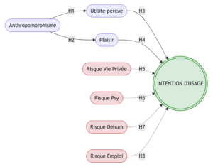
Le PLS transforme ces réponses en un score synthétique (« variable latente »), puis teste si ce score influence d’autres concepts comme l’Intention d’utilisation. C’est ça, un modèle PLS : des flèches de causalité entre des concepts abstraits, tous construits à partir de vos questions de terrain.
Comment ça fonctionne, étape par étape
Les 4 critères-clés que le code calcule pour vous
Alpha de Cronbach
Mesure si les questions d’un même bloc sont cohérentes entre elles. Si le score est faible, vos répondants n’ont pas compris les questions de la même façon.
Seuil ≥ 0,70AVE
Average Variance Extracted : vérifie que vos questions capturent bien le concept qu’elles sont censées mesurer, et non du bruit aléatoire.
Seuil ≥ 0,50VIF
Variance Inflation Factor : s’assure que deux variables ne font pas « double emploi ». Un VIF élevé rend les coefficients instables et peu fiables.
Seuil < 5,00Matrice HTMT
Test le plus sévère : prouve que deux concepts sont bien distincts dans l’esprit du répondant. Si le score est trop proche de 1, les concepts se confondent.
Seuil < 0,85 – 0,90Avant de lancer le code : étape cruciale
Le script Python lit vos données depuis un fichier Excel. Vous devez impérativement modifier le nom du fichier à la ligne 10 du code selon votre groupe :
| Votre groupe | Nom du fichier à inscrire dans le code |
|---|---|
| L3 MRC et IHR | BASE-MRC-IHR.xlsx |
| L3 MHR Hébergement | BASE-Hbgt.xlsx |
| L3 MHR Restauration | BASE-MHR-Rest.xlsx |
Attention : Si le nom ne correspond pas exactement (majuscules, tirets, extension…), le programme affichera une erreur “File Not Found” et ne pourra pas démarrer.
Téléchargement des bases de données
Téléchargez le fichier Excel correspondant à votre groupe et importez-le dans votre session Google Colab :
Le code Python (Version Expert)
Ce code calcule automatiquement les Coefficients, le Bootstrap, le VIF, l’AVE et la matrice HTMT. Copiez ce script dans Google Colab :
import pandas as pd
import numpy as np
from sklearn.model_selection import cross_val_predict
from sklearn.linear_model import LinearRegression
from sklearn.metrics import mean_squared_error, r2_score
import statsmodels.api as sm
from statsmodels.stats.outliers_influence import variance_inflation_factor
from tqdm import tqdm

# ==========================================
# === 1) CONFIGURATION ET LECTURE DU FICHIER
# ==========================================
FILE_PATH = "/content/BASE-MRC-IHR.xlsx"
SHEET_NAME = "BASE"

df = pd.read_excel(FILE_PATH, sheet_name=SHEET_NAME)
print(f"Fichier chargé : {FILE_PATH} | Taille : {df.shape}")

# Blocs de mesure — construits impliqués dans H1–H6 + H_Dehum + H_Emploi
blocks = {
    "Anthropomorphisme": ["ANT1","ANT2","ANT3","ANT4","ANT5"],
    "Utilite": ["UTIL1","UTIL2","UTIL3","UTIL4","UTIL5","UTIL6","UTIL7"],
    "Plaisir": ["PLAIS1","PLAIS2","PLAIS3","PLAIS4"],
    "RisqueViePrivée": ["RCONTETH1","RCONTETH2","RCONTETH3","RCONTETH4"],
    "RisquePsy": ["RPSY1","RPSY2","RPSY3"],
    "RisqueDehum": ["RDEHUM1","RDEHUM2","RDEHUM3","RDEHUM4","RDEHUM5"], # NOUVEAU
    "RisqueEmploi": ["RPEMP1","RPEMP2","RPEMP3","RPEMP4","RPEMP5"], # NOUVEAU
    "Intention": ["INT1","INT2","INT3","INT4"]
}

# Topographie du réseau (Inner Model)
# Ajout de RisqueDehum → Intention et RisqueEmploi → Intention
base_relations = [
    ("Anthropomorphisme", "Utilite"), # H1
    ("Anthropomorphisme", "Plaisir"), # H2
    ("Plaisir", "Intention"), # H3
    ("Utilite", "Intention"), # H4
    ("RisqueViePrivée", "Intention"), # H5
    ("RisquePsy", "Intention"), # H6
    ("RisqueDehum", "Intention"), # H_Dehum — NOUVEAU
    ("RisqueEmploi", "Intention") # H_Emploi — NOUVEAU
]

# Modèle Structurel (Équations)
# Intention intègre désormais les deux nouveaux prédicteurs de risque
equations = {
    "Utilite": ["Anthropomorphisme"], # H1
    "Plaisir": ["Anthropomorphisme"], # H2
    "Intention": ["Plaisir", "Utilite", "RisqueViePrivée", "RisquePsy",
                  "RisqueDehum", "RisqueEmploi"] # H3–H6 + Dehum + Emploi
}

all_items = [item for sublist in blocks.values() for item in sublist]
df_items = df[all_items].dropna().copy()

# ==========================================
# === 2) L'ALGORITHME ITERATIF PLS-SEM
# ==========================================
def run_pls_sem(data_raw, blks, relations, max_iter=100, tol=1e-5):
    X = (data_raw - data_raw.mean()) / data_raw.std()
    lv_names = list(blks.keys())
    C = pd.DataFrame(0.0, index=lv_names, columns=lv_names)

    for s, t in relations:
        if s in lv_names and t in lv_names:
            C.loc[s, t] = 1.0
            C.loc[t, s] = 1.0

    Y = pd.DataFrame({lv: X[items[0]] for lv, items in blks.items()})

    for _ in range(max_iter):
        Y_old = Y.copy()
        E = Y.corr() * C
        Z = Y.dot(E)
        Z = (Z - Z.mean()) / Z.std()

        W = {}
        for lv, items in blks.items():
            w = X[items].apply(lambda col: col.cov(Z[lv]))
            w = w / np.linalg.norm(w)
            W[lv] = w
            Y[lv] = X[items].dot(w)

        Y = (Y - Y.mean()) / Y.std()
        if np.abs(Y - Y_old).max().max() < tol:
            break

    Loadings = {lv: X[items].apply(lambda col: col.corr(Y[lv])) for lv, items in blks.items()}
    return Y, W, Loadings

Y_final, W_final, L_final = run_pls_sem(df_items, blocks, base_relations)

# La fonction est conservée mais ne crée plus de variables d'interaction
def calculate_inner_variables(Y_df):
    return Y_df.copy()

Y_complet = calculate_inner_variables(Y_final)

# ==========================================
# === 3) CALCUL DES CRITÈRES DE QUALITÉ
# ==========================================
qualite_list = []
loadings_df_list = []

for lv, loadings in L_final.items():
    for item, l_val in loadings.items():
        loadings_df_list.append({"Construit": lv, "Item": item, "Loading_Wold": l_val})

    n = len(blocks[lv])
    corr_matrix = df_items[blocks[lv]].corr()
    avg_corr = corr_matrix.values[np.triu_indices(n, k=1)].mean() if n > 1 else 1.0
    alpha = (n * avg_corr) / (1 + (n - 1) * avg_corr) if n > 1 else 1.0

    ave = np.mean(loadings**2)
    sum_l = np.sum(loadings)
    sum_e = np.sum(1 - loadings**2)
    cr = (sum_l**2) / (sum_l**2 + sum_e)

    qualite_list.append({"Variable": lv, "Cronbach_Alpha": alpha, "Composite_Reliability": cr, "AVE": ave})

df_loadings = pd.DataFrame(loadings_df_list)
df_qualite = pd.DataFrame(qualite_list)

X_std = (df_items - df_items.mean()) / df_items.std()
latent_names = list(blocks.keys())
htmt_df = pd.DataFrame(index=latent_names, columns=latent_names, dtype=float)

for i, b1 in enumerate(latent_names):
    for j, b2 in enumerate(latent_names):
        if i == j:
            htmt_df.iloc[i,j] = 1.0
        elif i < j:
            items1, items2 = blocks[b1], blocks[b2]
            hetero_mean = X_std[items1 + items2].corr().loc[items1, items2].values.mean()
            mono1 = X_std[items1].corr().values[np.triu_indices(len(items1), k=1)].mean() if len(items1)>1 else 1.0
            mono2 = X_std[items2].corr().values[np.triu_indices(len(items2), k=1)].mean() if len(items2)>1 else 1.0
            htmt_val = abs(hetero_mean / np.sqrt(max(0.0001, abs(mono1 * mono2))))
            htmt_df.iloc[i,j] = htmt_val
            htmt_df.iloc[j,i] = htmt_val

fl_matrix = Y_final.corr()
for b in latent_names:
    fl_matrix.loc[b, b] = np.sqrt(df_qualite.loc[df_qualite['Variable'] == b, 'AVE'].values[0])

# ==========================================
# === 4) MODELE STRUCTUREL (R², f², VIF)
# ==========================================
results_inner = {y: sm.OLS(Y_complet[y], sm.add_constant(Y_complet[xs])).fit() for y, xs in equations.items()}

structurel_data = []
for dep, preds in equations.items():
    X_mat = sm.add_constant(Y_complet[preds])
    R2_incl = results_inner[dep].rsquared

    for i, p in enumerate(preds, start=1):
        vif = variance_inflation_factor(X_mat.values, i)
        preds_excl = [x for x in preds if x != p]
        R2_excl = 0 if not preds_excl else sm.OLS(Y_complet[dep], sm.add_constant(Y_complet[preds_excl])).fit().rsquared
        f2 = (R2_incl - R2_excl) / (1 - R2_incl)

        structurel_data.append({
            "Variable_Dep": dep, "Predictor": p,
            "Coefficient": results_inner[dep].params[p],
            "f2": f2, "VIF": vif
        })
df_structurel = pd.DataFrame(structurel_data)

# ==========================================
# === 5) BOOTSTRAPPING (t-values)
# ==========================================
def run_bootstrap(data_raw, n_boot=500):
    rng = np.random.default_rng(123)
    boot_coefs = []
    for _ in tqdm(range(n_boot), desc="Bootstrapping PLS"):
        sample = data_raw.sample(len(data_raw), replace=True, random_state=rng.integers(0, 100000))
        Y_boot, _, _ = run_pls_sem(sample, blocks, base_relations, max_iter=30)
        Y_boot_comp = calculate_inner_variables(Y_boot)
        row = {}
        for dep, preds in equations.items():
            res = sm.OLS(Y_boot_comp[dep], sm.add_constant(Y_boot_comp[preds])).fit()
            for p in preds:
                row[(dep, p)] = res.params[p]
        boot_coefs.append(row)
    return pd.DataFrame(boot_coefs)

boot_df = run_bootstrap(df_items, n_boot=500)
boot_std = boot_df.std()
boot_ci = boot_df.quantile([0.025, 0.975]).T
boot_ci.columns = ["CI_lower", "CI_upper"]

df_structurel["t-value"] = df_structurel.apply(
    lambda r: abs(r["Coefficient"] / boot_std[(r["Variable_Dep"], r["Predictor"])]), axis=1
)
df_structurel["p-value"] = [results_inner[r["Variable_Dep"]].pvalues[r["Predictor"]] for _, r in df_structurel.iterrows()]
df_structurel["Significatif_t"] = df_structurel["t-value"] > 1.96

# ==========================================
# === 6) FIT GLOBAL (SRMR) & MACHINE LEARNING (Q² / PLSpredict)
# ==========================================
# --- SRMR ---
R_obs = df_items.corr()
R_implied = pd.DataFrame(np.eye(len(all_items)), index=all_items, columns=all_items)
lv_corr = Y_complet[latent_names].corr()

item_lv_map = {item: lv for lv, items in blocks.items() for item in items}
item_loading_map = {item: L_final[lv][item] for lv, items in blocks.items() for item in items}

for i in range(len(all_items)):
    for j in range(i+1, len(all_items)):
        it1, it2 = all_items[i], all_items[j]
        lv1, lv2 = item_lv_map[it1], item_lv_map[it2]
        r_imp = item_loading_map[it1] * item_loading_map[it2] * lv_corr.loc[lv1, lv2]
        R_implied.loc[it1, it2] = r_imp
        R_implied.loc[it2, it1] = r_imp

diff = R_obs.values - R_implied.values
mask = np.triu(np.ones(diff.shape), k=1).astype(bool)
srmr_value = np.sqrt(np.mean(diff[mask]**2))

df_srmr = pd.DataFrame([{
    "Metric": "SRMR Global", "Valeur": srmr_value,
    "Seuil": "< 0.08 (Idéal) / < 0.10 (Acceptable)",
    "Statut": "Excellent" if srmr_value < 0.08 else ("Acceptable" if srmr_value < 0.10 else "À revoir")
}])

# --- Q² (10-Fold CV sur modèle structurel) ---
lr = LinearRegression()
q2_list = []
for dep, preds in equations.items():
    y_pred_cv = cross_val_predict(lr, Y_complet[preds], Y_complet[dep], cv=10)
    q2_list.append({
        "Variable Endogène": dep,
        "R2_In_Sample": results_inner[dep].rsquared,
        "Q2_Predictive_Relevance": r2_score(Y_complet[dep], y_pred_cv)
    })
df_q2 = pd.DataFrame(q2_list)

# --- PLSpredict (Items endogènes - Uniquement sur l'Intention) ---
plspredict_list = []
endog_targets = ["Intention"]

for target_lv in endog_targets:
    for item in blocks[target_lv]:
        y_item = df_items[item]

        exog_lvs = equations[target_lv]
        exog_items = list(set([it for ex in exog_lvs if ex in blocks for it in blocks[ex]]))
        X_item_lm = df_items[exog_items] if exog_items else df_items.drop(columns=[item])

        y_pred_lm = cross_val_predict(lr, X_item_lm, y_item, cv=10)
        y_pred_naive = np.full_like(y_item, y_item.mean())

        rmse_lm = np.sqrt(mean_squared_error(y_item, y_pred_lm))
        rmse_naive = np.sqrt(mean_squared_error(y_item, y_pred_naive))
        q2_predict_item = 1 - (mean_squared_error(y_item, y_pred_lm) / mean_squared_error(y_item, y_pred_naive))

        plspredict_list.append({
            "Cible": target_lv, "Indicateur": item,
            "RMSE_Machine_Learning (LM)": rmse_lm, "RMSE_Moyenne_Naive": rmse_naive,
            "Q2_predict": q2_predict_item,
            "Pouvoir_Predictif": "Fort" if rmse_lm < rmse_naive else "Faible"
        })
df_plspredict = pd.DataFrame(plspredict_list)

# ==========================================
# === 7) EXPORT EXCEL EXHAUSTIF
# ==========================================
filename = "Resultats_Analyse_Expert_PLS.xlsx"
with pd.ExcelWriter(filename) as writer:
    df_structurel.to_excel(writer, sheet_name='Paths_tvalue_f2_VIF', index=False)
    df_srmr.to_excel(writer, sheet_name='Fit_SRMR', index=False)
    df_q2.to_excel(writer, sheet_name='Q2_Relevance_Structurelle', index=False)
    df_plspredict.to_excel(writer, sheet_name='PLSpredict_Items', index=False)
    df_loadings.to_excel(writer, sheet_name='Loadings_Items', index=False)
    df_qualite.to_excel(writer, sheet_name='Fiabilite_Mesure', index=False)
    fl_matrix.to_excel(writer, sheet_name='Fornell_Larcker')
    htmt_df.to_excel(writer, sheet_name='Validite_HTMT')

print(f"Modèle étendu exécuté avec succès. Fichier généré : {filename}")
Comment lire votre fichier Excel ?
Le fichier « Resultats_Analyse_Expert_PLS.xlsx » contient plusieurs onglets. Voici comment interpréter chacun d'eux :
Pour valider vos hypothèses. Si la colonne « Significatif » affiche True, l'impact causal est réel et statistiquement prouvé.
Vérifiez que l'AVE > 0,50 et l'Alpha de Cronbach > 0,70 pour chaque variable latente.
Tous les VIF doivent être inférieurs à 5. Au-delà, les résultats sont instables et peu interprétables.
Chaque score doit être < 0,85 ou 0,90 pour prouver que vos concepts sont bien distincts les uns des autres.
Indique la part de variance expliquée par votre modèle. Plus proche de 1, plus votre modèle est puissant.
Mesure la pertinence prédictive : votre modèle fait-il mieux que de simplement prédire la moyenne ?
Accès aux résultats par groupe
Sélectionnez votre groupe ci-dessous pour accéder directement à la page de consultation de vos résultats :